We need to first figure out the problem we are dealing with falls under which category.
It has to be one of the 4 categories.
We will try to understand each one of these categories in detail. But we will go in the reverse order. We will begin with the reinforced learning problem.
4. Reinforced Learning Problem
As per Wikipedia, "Reinforcement learning is an area of machine learning concerned with how intelligent agents ought to take actions in an environment in order to maximize the notion of cumulative reward."
This is yet another simple explanation of RL from GeeksforGeeks, "It is about taking suitable action to maximize reward in a particular situation. It is employed by various software and machines to find the best possible behavior or path it should take in a specific situation. Reinforcement learning differs from the supervised learning in a way that in supervised learning the training data has the answer key with it so the model is trained with the correct answer itself whereas in reinforcement learning, there is no answer but the reinforcement agent decides what to do to perform the given task. In the absence of a training dataset, it is bound to learn from its experience."
Reinforced Learning is used in video games for testing & research. Reinforcement Learning in current days is also used in highly complex applications such as self driving cars, news recommender systems, gaming (Alpha Go Zero), marketing & advertising etc.
The system works as shown below.
The python libraries that are used in reinforcement learning are, Coach, Tensorforce, Stable Baseline etc.
3. Semi supervised Learning
Semi supervised learning as the name suggests deals with both labeled & unlabeled data.
Labeled data has to be of very small amount.
Unlabeled data is the majority in Semi supervised problems.
Examples :
Speech Analysis
Internet Content Classification
DNA Sequence Classification
1. Supervised Learning:
When we are dealing with labeled data we call the problem as a supervised learning problem.
For every input x, there has to be an output. And if that output is continuous then the problem is a Regression Problem. If that output is discrete then we call it a Classification Problem.
1.1 Regression Problem:
There can be various types of regression problems. They are,
Linear regression
Ridge regression
Neural Network regression
Lasso regression
Decision Tree regression
Random Forest regression
KNN regressor
SVR (Support Vector Regressor)
1.1.1 Linear Regression:
Linear regression gives the statistical relation between two (or more) variables. Statistical relation is not exactly accurate.
The opposite of Statistical relation is Deterministic relation. Deterministic relation is accurate.
An example to understand would be, the relation between temp in degree Celsius & degree Fahrenheit. There is a certain formula so this relation is always accurate & hence deterministic.
In case of linear regression, the idea is always to obtain the best fit line that represents the data.
We also try to keep the prediction error as low as possible.
Prediction error is calculated by taking sum of square value (because taking normal difference will cancel out positive errors and negative errors)
And the statistical relation we are talking about looks like this (the example is for 1 independent variable):
Model Evaluation: (Goodness of fit)
For model evaluation we use a metric called R square. R Square indicated to what extent the variance in independent variable explains the variance of the output variable. The R square value ranges between 0 & 1.
R Sq of 0 = Predictors have no influence on the predicted values
R Sq of 1 = Predictor totally influences the predicted values
When implementing linear reg in python the "model.score()" will give us the R square value.
How to optimize a linear regression?
Do note that there exists NO Hyperparameters in Standard Linear Regression( also called OLS / Normal linear Regression).
However, in case of LASSO or Ridge Regression, we can use Learning Rate / Shrinkage Factor as hyperparameter.
So because of it's linear nature, there can be only one best line with minimum residual / error / bias.
The idea is to minimize he error and we end up with that one best line.
Disadvantages of Linear Regression:
Linear regression is too simple. It fails to capture any non linear relation.
Solution : We may try using polynomial regression.
But, in Polynomial Regression we may run into a problem of overfitting. (or underfitting in case of OLS).
To deal with this, we use LASSO Regression (Also called L1 Regularization) or Ridge Regression (Also called the L2 Regularization).
For LASSO in sklearn, - Lasso( α = some hyp value )
For Ridge Reg in sklearn, - Ridge( α = some hyp value )
In both Lasso & ridge regression, a penalty is added to the loss function.
1.1.2 SVR (Support vector Regressor):
How kernel trick works in SVM can be understood from this
What Kernel trick does is, it increases the dimension of Data so that a non linear problem becomes linear, meaning there can be a linear decision boundary (possibly a hyperplane) which previously would have been a non linear boundary.
Feature independence.
Demerit:
Not satisfactory result for large dataset
Cant handle outliers
Doesn't work if classes are overlapping
1.2 Classification
Some of the classification techniques are Logistic Regression, Naive Bayes, Stochastic Gradient Descent, KNN, SVM, Decision Tree.
1.2.1 Logistic Regression:
Assumptions: All features are independent.
Logit is a binary classifier.
In sklearn it has a method named, LogisticRegression()
Just like Linear Regression, Logistic Regression also has no hyperparameters to tune.
|
“Random State” in all sklearn algorithms is used to pass a value for
degree of randomness to a random number generator. It doesn’t have any
functionality associated with how the algorithm actually works. So When we
pass Random State as a parameter, please remember that this is not a hyper
parameter and is not a part of the algo.
|
Though it is a classification problem it's similarity with the linear regression equation got it the "regression" in it's name. let's see how the equation for logistic regression looks similar to that of the linear regression.
The expression takes the form,
It's a linear method. But the linear output is transformed later using a logistic function.
Accuracy is at times misleading & hence we use the other metrics such as Precision, Recall & F1 Score.
Buy why is accuracy misleading?
One reason is there could be imbalance in the data & that may cause a very misleadingly high accuracy even if the model is actually doing poorly.
Advantages:
You can use model coeff as indicators of feature importance.
Simple
Linear
Less prone to overfitting.
Disadvantages:
If Number of rows < Number of features - Overfitting
Linear boundaries - Doesn't capture the non linearities. Most problems in real world are non linear.
- PS: There are no hyper parameters to tune for Logistic Regression. However there are solvers we have to pass as parameters. They are newton-cg, SAG, SAGA, lbfg to name a few. These all represent different cost functions & are useful in different scenarios. SAG & SAGA are useful when we are dealing with large datasets with a lot of sparsity. Likewise each one has it's advantages & disadvantages. We will explore those further when we are working on a problem.
1.2.2 Naive Bayes:
Naive Bayes works on the same principle of Bayes theorem but with one naive assumption that all features are absolutely independent of each other. Naive it is, because in real world there is no such absolute independence among all the variables. Still making this minor assumption makes life a lot easier.
In sklearn we have a method to implement naive bayes i.e. GaussianNB()
One area where Naive Bayes is extensively used is text classification.
1.2.3 Stochastic Gradient Descent
This is also linear. It works on large datasets. This supports many loss functions.
Advantage: linear, Simple, Fast
Disadvantage: Sensitive to feature scaling,
needs many hyper parameters
1.2.4 KNN:
Works for non linear classification.
Works for large datasets.
Robust on outliers.
Why is this called a lazy learner?
Because it doesn't actually construct any internal model. It works by voting among neighbors.
in sklearn, there is a method for this.
KNeighborsClassifier( n_neighbors = k )
KNN is a non parametric method. So no assumptions are made.
But it assumes all data points lie within the feature space.
Demerit:
High computation cost as it computes distances (commonly Euclidean distance)
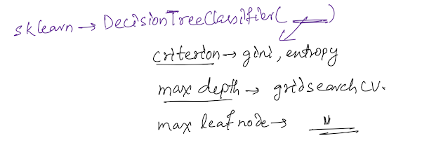
1.2.5 Decision Tree:
Decision Tree is non parametric. So no assumptions are made. DT also doesn't require to scale the data.
In Decision Tree all the features are preferred to be categorical. Though it works on continuous features too, it in a way bins the continuous features to handle it.
In case of continuous features, a threshold is set by the algo and then based on the threshold, splitting is done.
Multiclass classification
easy readability (set of if else)
not impacted by outliers
Non linear classification
Feature importance can be found from the tree
Disadvantage:
small change - affects the whole tree
class imbalanced data - underfit tree
Various varieties of Decision Tree:
ID3
C4.5
CART
CHAID
MARS
Unsupervised Learning
Unlike supervised learning, unsupervised learning extracts limited features from the data, and it relies on previously learned patterns to recognize likely classes within the dataset. Instead of trying to make predictions, unsupervised learning algorithms will try to learn the underlying structure of the data.
Most common types of unsupervised learning are k-means, hierarchical clustering, and principal component analysis.
Principal Component Analysis:
PCA is a method where we find out a lower dimensional representation of the original high dimensional data without losing much of the information. We lose some of the variance in the data in the dimensionality reduction process but the problem then becomes way more easier to deal with. It becomes much lesser computationally expensive.
There are different types of PCA. Such as, incremental PCA, nonlinear variants such as kernel PCA, and sparse variants such as sparse PCA.
SVD:
Another popular approach is to reduce the rank of the original matrix of features to a smaller rank such that the original matrix can be recreated using a linear combination of some of the vectors in the smaller rank matrix. This is known as SVD.


