

Step 2: Data Pre-processing:

(i) Check for inconsistencies.
Here we check for inconsistencies in the data.
At times due to human error some entries in a tabular data could be erratic. In the age column someone might have entered the Surname or a similar human error could happen every now and then. If the data is collected using a survey form and someone knowingly tried to fill in absurd answers. Or it could happen that while extracting a report using some SQL query a wrong query resulted in duplicate rows. These are a few possible causes why data inconsistencies occur.
We will discuss how we can check this issue while working with python in a Jupyter Notebook. A simple pandas .info() method applied on the dataframe shows us the datatypes of all available columns.

From this we can also check if any column has missing column name. If so has happened we can try naming the particular column. We can do .rename() as below.
If we observe an int datatype for a column which was supposed to be string or float we can take appropriate actions to make the necessary correction. What action is to be taken depends upon the problem at hand. In some cases simply changing a datatype will do, in other cases we may have to make changes in the manner in which our data is being tapped at the source or the solution could be any one of the thousand different possibilities.
(ii) Missing value treatment.
This is a very common problem. In almost every problem in real life, we will need to treat the missing rows before doing analysis on the dataset. First we check the count of missing entries. In python it can be done with df.isna().sum() or df.isnull().sum().

Now that we have the count, how do we treat the missing values?
(a) If the count is small and so insignificant that we can afford to lose it then dropping the missing values can help us get rid of this problem.
(b) However in certain cases such as sensitive government data, medical records etc, we can not afford to drop even a small portion of the data. In that case we try to replace the NaN values with a substitute. In the above case we see 92 missing values from 20,000 entries which is a small portion (0.46%) of the entire data. If we observe that a significant portion say 40-50% of the record are missing then replacing missing records with any substitute is not a good idea.
Usually we replace the missing rows with some substitute value so that we can perform our statistical analysis. This process of replacing missing values with some other substitute is called imputation. We have 3 basic imputation methods at our disposal i.e. imputation by mean value, median value or mode value of the entire column. Other than these 3, there are some sophisticated missing value/NaN value treatments as well. We will discuss them further.
How do we know which is the right method of imputation?
The answer is, if we are dealing with a numerical continuous column, we can replace by mean of the entire column.
However the problem with mean value imputation is that, the mean of a distribution is influenced by outliers. So suppose a column "Student age" has one outlier value of 3000, then that presence of an impossible age entry (i.e. the outlier) will nudge the mean of the whole column way up than what the mean value would have been had there be no outlier. Hence imputing by mean may not be a good idea always. We will only use this method of imputation when we are sure that our column doesn't have any outliers present.
In case we know we have outliers in the data, then imputation by median value can be used. Median doesn't get influenced by the presence of outliers.
Suppose we are dealing with categorical data and not numeric ones, in that case we can not find mean of categorical entries. In such cases imputing with the mode value i.e. the most frequent occurrence will be a good idea.
In python, we can achieve missing value imputation by using the .fillna() method as follows. Here we are trying to impute the missing values in 'bmi' column using median.
df['bmi'] = df['bmi'].fillna(df['bmi'].median())
Apart from imputation by mean, median & mode value, there are some other better imputation methods such as KNN imputer etc.
(iii) Encode the categorical columns:
The third step in data preprocessing is to perform encoding. If we have categorical data then performing statistical analysis over it could be challenging. Converting the categorical values to numeric ones makes life easier. For example if we have Gender column with values as "Female", "Male" & "Other", we can encode these as 0, 1 & 2 respectively. Likewise we could also create dummy variables in order to perform encoding. Dummy variables is an interesting concept. We encourage you to check out this small article on dummy variables to understand how it works.
Of the various way to encode categorical values, there are the three commonly used methods.
(a) Using dummy variabales.
You may like reading : Dummy variables
(b) Using Ordinal encoding:
In python you can use the OrdinalEncoder from Sklearn library to perform encoding.
(c) Using One Hot Encoding:
For categorical variables where there exists no ordinal relationship, performing a normal ordinal encoding may put us in trouble. Applying ordinal encoding in such case will cause the model to assume a natural ordering between categories which may result in erratic analysis & predictions. In this case, a one-hot encoding comes to rescue. Here the integer encoded variable is removed and one new binary variable is added for each unique integer value in the variable so that we end up with only 1 & 0s as entries (binary values).
(iv) Feature Scaling:
In some cases we may feel the need to perform feature scaling on our dataset. What feature scaling does is, it brings all the features to comparable ranges. Doing so has it's own advantages too.
Most algorithms perform better & give better accuracies when features are scaled.
What is the need you may still ask. It is a bit of a trouble when you have to work with a dataset where values of one column ranges between -500 and +500 & that of another between 0 to 7. You will find it difficult to make plots or perform bivariate analysis using those two features. But you remember your friend saying that day that you do not need to do feature scaling because you can always use algorithms like decision tree or such and they will work just fine without feature scaling. Yes your friend is right. But what about the other algorithms which do work well when features are scaled. So in a nutshell, it is wise to scale the features before we initiate our analysis.
Now that we are kind of convinced that it's a good idea to get the features scaled, we would like to know what are the methods we can use to perform feature scaling.
We will discuss two popular methods of feature scaling. Normalization & Standardization.
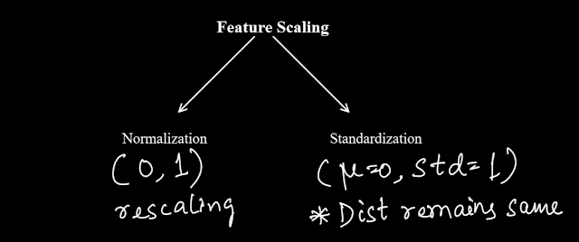
(a) Normalization:
Normalization is when the distribution is mapped to a range between 0 & 1.
(b) Standardization:
Standardization is when a rescaling is done to make the mean of the dist as 0 and std as 1. Please note that standardization doesn't alter the original distribution. It doesn't make the distribution normal. It only rescales all the values to make mean 0 and std 1.
(v) Outlier treatment:
Outliers are the odd, absurd or abnormal entries in he data which could have appeared due to an error or could indicate some real data points which exhibit behavior that doesn't fit in with the rest of the distribution. It is important to be aware of any presence of outliers in our data. An outlier doesn't necessarily mean it's a wrong entry, though wrong entries or error in reading from a faulty sensor or instrument do cause outliers to appear. An example of this could be in a dataset showing incomes of residents in a county where Jeff Bezos lives, the income of Jeff Bezos will be significantly higher than the rest of the population and hence that lone entry might appear to be an outlier. But as we know, it definitely doesn't mean there has been a wrong entry in the data. So while handling outliers we have to be careful and take all sorts of practicalities into consideration.
How do we detect outliers in data?
There is no one proven way to check that. Several techniques are used depending upon the problem. We will discuss some of the common widely used methods. One of those is the IQR method.

(a) Inter Quartile Range for outlier detection:
This is a very popular method for detecting outliers. In a distribution we find out the first quartile (Q1) & the third quartile(Q3). We find out the IQR by subtracting Q1 from Q3. Then we establish a range between Q1-1.5*IQR & Q3+1.5*IQR. Any data point that lies within this range is termed an inlier and anything that falls beyond this range is termed an outlier.
This link from Khan Academy explains it in detail.
Clearly this method is not robust but in most cases it gets the job done.
(b) Boxplots:
Another way to detect outliers is by using boxplot. This method is no different from the previous method. It used the same calculations as in IQR method but it presents the same as a box & whisker plot so that we can notice the outlier points visually. The below plot is an example of a boxplot.

(c) Z Score / Standard Score:
For all data points z-scores are calculated using the formula,
Z score of a data point = ( Data point - Mean ) / std
This gives a score for each data point. A threshold is set (usually 3).
If the score is > threshold, then the entry is an Outlier.
If the score is < threshold, then the entry is not an Outlier.
(d) One Class Classification:
One class classification methods are more robust in detecting outliers as compared to the traditional method we discussed so far. There are several one class classification algorithms. We have discussed some of them briefly here.

In sklearn library we can find each of these One Class Classifiers.
One Class SVM:
In sklearn there is a method named OneclassSVM( nu = 0.03 )
hyperparameter - nu , if set at 0.03 means, 3% will be termed as outliers.
Isolation Forest:
This is a tree based outlier detection classifier.
Python Syntax is: model = IsolationForest( contamination = 0.01 )
hyperparameter is contamination & it's value we have to know.
Local Outlier Factor (LOF):
LOF works like the K Nearest neighbors.
Each data point is assigned a local neighborhood score. This score tells how isolated the point is or in other words, how likely it is an outlier, based on its local neighborhood.
The higher the score, the more likely the point is to be an outlier.
In python, we can use this by typing
clf = LocalOutlierFactor( contamination = 0.01 )
The LOF method has one demerit.
It only works with low dimensional data. If number of features goes up = LOF fails.
(e) HBOS:
HBOS stands for Histogram Based Outlier Score. The formula looks as below.

Steps to achieve this :-
1. histogram / Binning of continuous data

2. 1 / (binned data)
3. log (result)
4. sum all feature values to get an HBOS score. Store it in a new column.

Now apply any outlier detection method s.a. boxplot or z score to get the outlier row.

Now we have understood various methods to detect outliers present in the data.
There are several ways to deal with outliers. If they are found to be erratic entries we can consider dropping them altogether.
We also face scenarios where we can not afford to lose the other features of that same entry which contains outlier value in one of its features. We have discussed such scenarios before. In such cases imputation again comes to our rescue. Instead of dropping the row altogether, we can impute that outlier value with mean(), median() or mode().
Here we discussed all the steps involved in data pre-processing. It's not mandatory to go through all of these steps every time. It all depends upon the nature of the problem.
Once we are done with the pre-processing step, the next logical step to undertake is the Exploratory Data Analysis or EDA in short.
We will discuss EDA in the next post. Visit this link to learn about EDA.


